SRE and ML forecasting
Table of contents
- Introduction
- Our dataset
- Benefits of Using ML Models
- The ML Models of Our Experiment
- Code and Libraries
- The Dataset
- Preliminary fitting and validation results
- Visual Verification and Validation
- Conclusion
Introduction
In this second forecasting article, we will use the concepts introduced in our first article about SRE and forecasting, and attempt to expand our toolkit to include machine learning models in addition to the stochastic models presented in the previous article.
We will present the strengths and weaknesses of a collection of representative models, but the comparison will not be exhaustive by any means.
SRE data often contains recurring cycles, spikes, and noise, so it is natural to ask whether flexible ML regressors can capture patterns that ETS smooths over. The purpose is not to replace classical forecasting automatically, but to compare model families under the same train-and-validate procedure.
Our dataset
The Original Dataset
For the purposes of this comparison, we will reuse the same dataset used in the first article. This dataset came from a private GoToSocial instance and included logs over a month.
These logs were transformed to group errors into 886 hourly buckets. After the analysis presented in the previous article, ETS with additive trend and additive weekly seasonality emerged as the best practical forecasting model after rejecting obvious overfitting candidates such as splines.
The original validation window contained 30 rows, and that ETS model previously showed useful predictive behavior on unseen data.
ML Data Transformation
In order to use ML models for forecasting, we need to transform our original data. We will use the buckets defined in the original article, but this dataset needs to be transformed even further in order to be usable by the ML models.
ML regressors do not understand time order by themselves, so lagged values and rolling summaries are what translate the time series into a tabular learning problem.
We will build lag features at 1, 2, 3, 6, 12, 24, 48, and 168 hours, plus rolling means and standard deviations over 3, 6, 24, and 168 hours.
This leads the ML training table to shrink from the full raw series to 717 usable rows: the 168-hour lag and rolling features require roughly one week of prior history before a row becomes usable.
It also aligns the ML models with our previous ETS model and our original data that demonstrated a 168-hour seasonality, so our ML model results can be compared directly with our ETS model results.
Benefits of Using ML Models
Having ML models as part of our forecasting toolkit is important because ML models can capture nonlinear patterns and feature interactions that a simpler time-series baseline like ETS may miss. In forecasting literature, ML is commonly used because it can exploit richer inputs, such as lag features, calendar effects, and external drivers, while still handling complex relationships in the data.
In more practical terms, an ML model does not rely 100% on the seasonality of an event, i.e. something happens every X amount of hours, but can also check localised state, i.e. an hour, or a few hours, or even a day earlier than the current time, and check if the event has started early, or if there is another nonlinear event taking place.
This is harder to express with a model such as ETS, which is a structured time-series framework built around error, trend, and seasonality. ETS can model trend and seasonal structure well, but it does not use the same flexible lag-feature table that ML models can exploit.
The ML Models of Our Experiment
In this experiment, we will use three ML models that are well established and fairly prominent in the ML world. These models are by no means the only ones available, but they are a good selection for highlighting the benefits of ML models in forecasting.
We will use:
- Ridge regression: A linear model with regularization, useful when many lag-based features are correlated and a simpler model may generalize better.
- Random forest: An ensemble of decision trees, useful for nonlinear interactions and threshold-like behavior in operational data.
- Histogram gradient boosting: A boosted tree model, useful because it can fit more complex nonlinear relationships than a single tree or a linear model.
We will compare all results with ETS, which showed the best performance among the forecasting models in our previous article.
Code and Libraries
For the purpose of this experiment, we will use Python 3.14.6 and the following libraries:
pandaswas used to load, clean, and reshape the hourly data.numpyhandled the numerical operations used for curve fitting and machine-learning steps.statsmodelswas used to build the ETS baseline.scikit-learnwas used to train the ML models.matplotlibwas used to generate the publication-ready PNG charts.
Python 3.14 is the current feature release series. Scikit-learn is an open-source machine learning library that supports tasks such as preprocessing, model fitting, and model selection.
The Dataset
You can download the original training dataset from here and the validation dataset from here if you want to replicate this experiment.
Preliminary fitting and validation results
After setting everything up we get the following results:
| Split | Model | Rows | MAE | RMSE | Status |
|---|---|---|---|---|---|
| Train | ETS | 717 | 38.98 | 60.52 | Baseline |
| Train | Ridge | 717 | 37.28 | 58.57 | Better (4.4% MAE, 3.2% RMSE) |
| Train | Random Forest | 717 | 25.22 | 42.94 | Better (35.3% MAE, 29.0% RMSE) |
| Train | HistGradientBoosting | 717 | 13.47 | 18.84 | Better (65.4% MAE, 68.9% RMSE) |
| Validation | ETS | 30 | 31.76 | 42.57 | Baseline |
| Validation | Ridge | 30 | 22.05 | 27.05 | Better (30.6% MAE, 36.5% RMSE) |
| Validation | Random Forest | 30 | 27.75 | 32.40 | Better (12.6% MAE, 23.9% RMSE) |
| Validation | HistGradientBoosting | 30 | 31.09 | 37.68 | Better (2.1% MAE, 11.5% RMSE) |
Results Discussion
In our previous article, we used MAE and RMSE to compare the behaviour of the various models. We will do the same here, using ETS as our baseline.
For ease of use, we can provide the definitions of MAE and RMSE here:
MAE is the average absolute error between the predicted and actual values, expressed in the same units as the data.
RMSE is similar, but it penalizes large errors more heavily, so it is more sensitive to outliers and occasional big misses.
In both cases, lower is better.
As we can see, the ML models are better than the baseline in almost all cases. The validation results reinforce the conclusion that we do get better performance from our ML models compared to the best-in-class ETS model from the previous article.
More Results Discussion
Based on the results above, we could be justified in concluding that we have a better method for forecasting than just using our best model from the previous article.
Is there anything else we can do to verify whether this is indeed the case or not?
The answer is yes: we can do visual validation, and hopefully this will give us a better understanding of our results and the strengths and weaknesses of our models.
Visual Verification and Validation
Here are all of our models when tested against the training dataset:
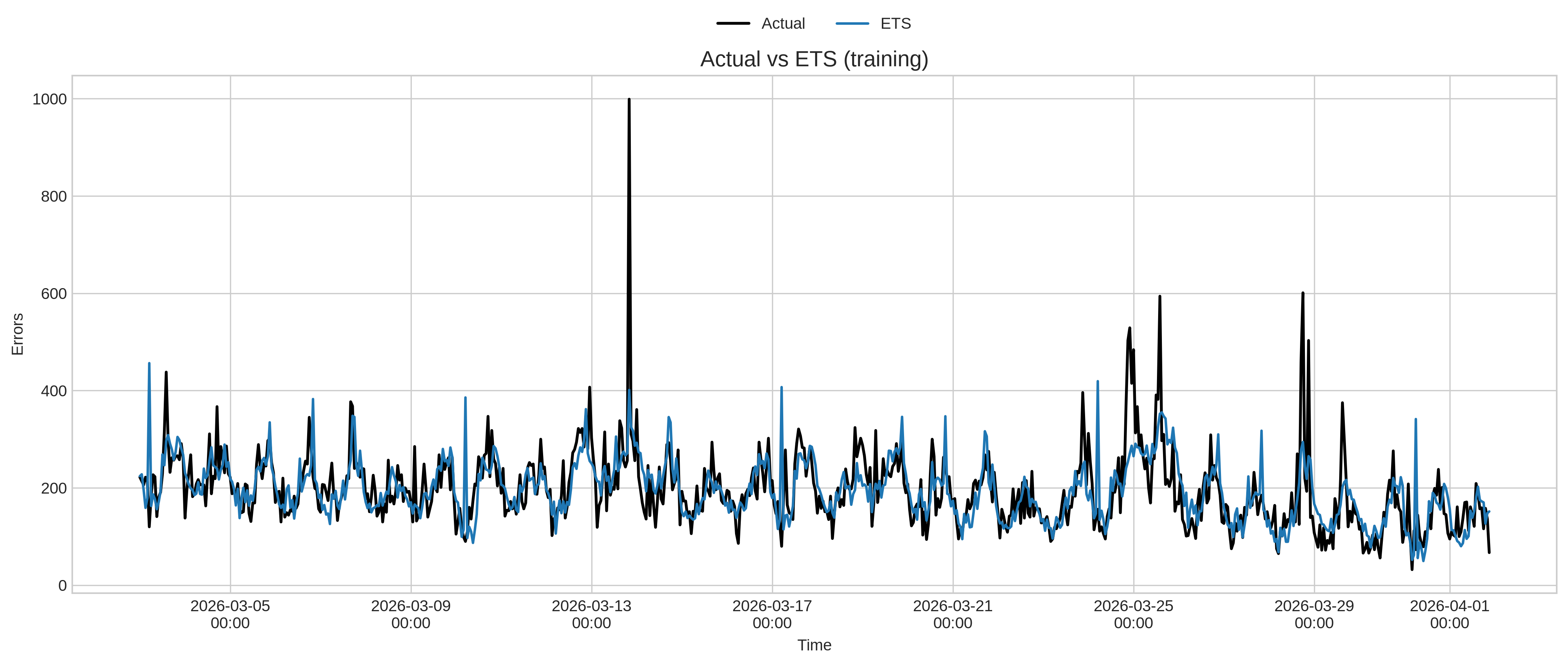
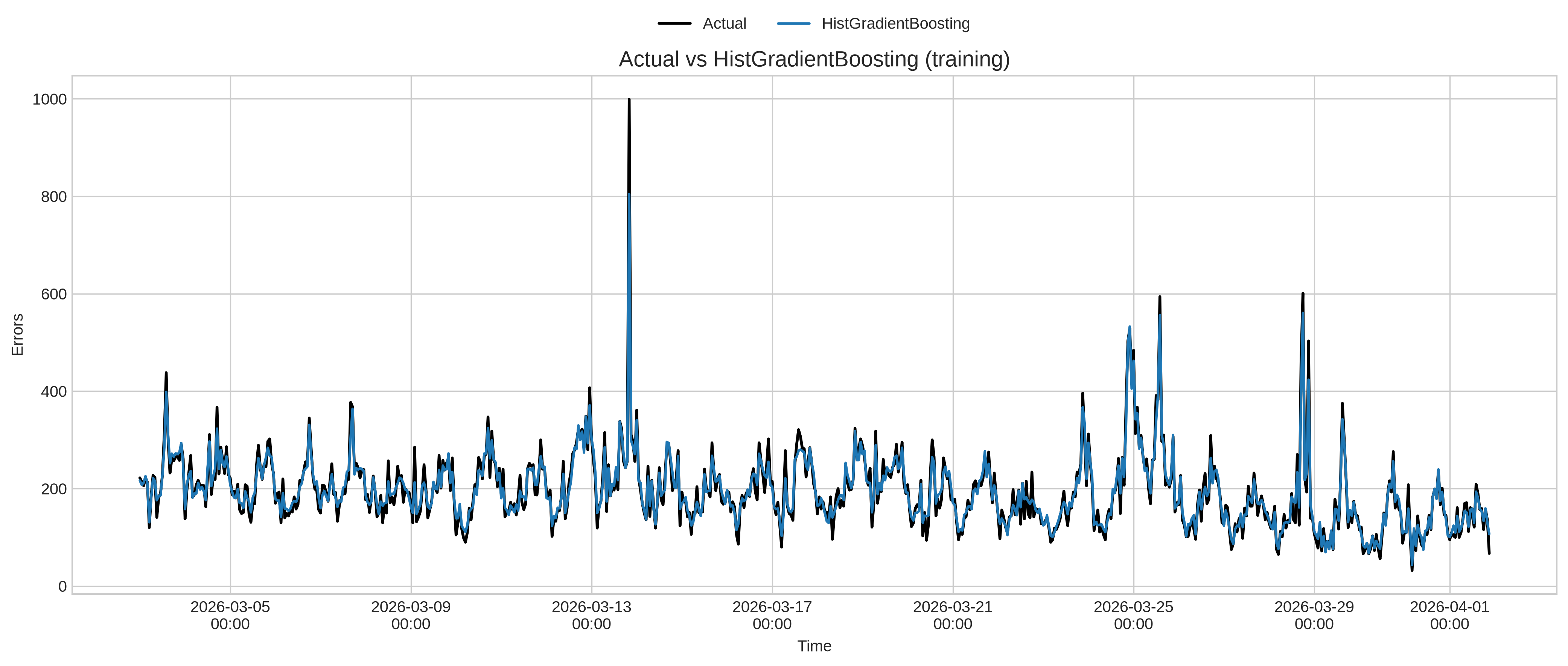
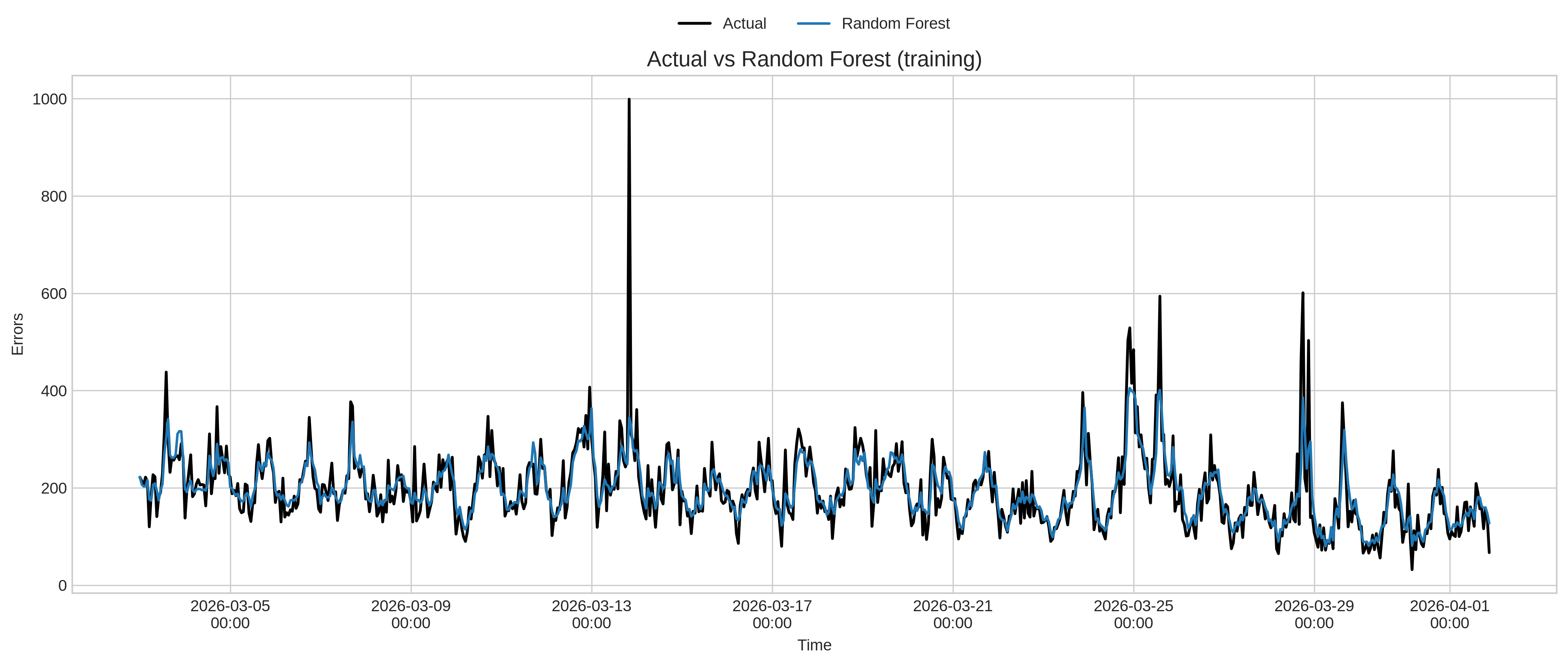
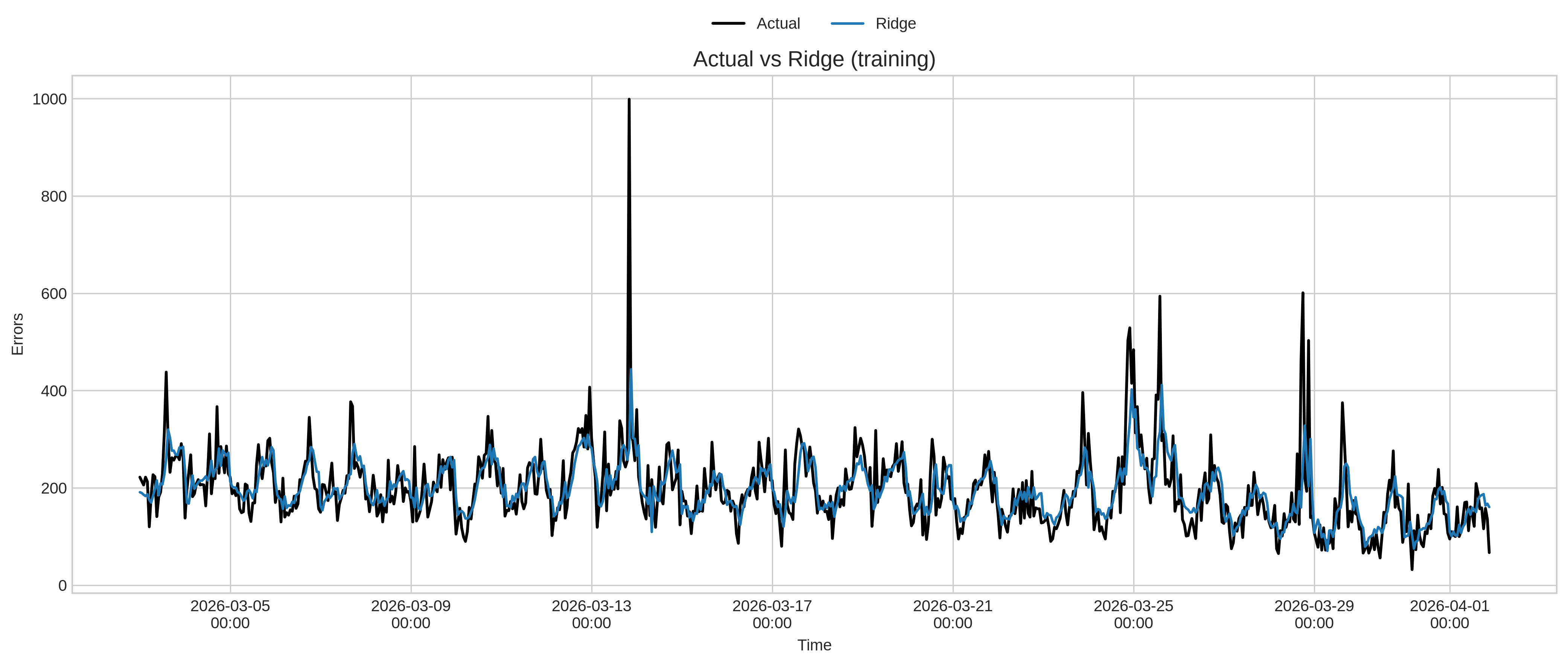
So far, so good: all of our models are performing quite well against the training dataset, but that is not enough. We need to verify how well they are doing against unknown data, not the data they were trained on.
Here are our results against the validation dataset:
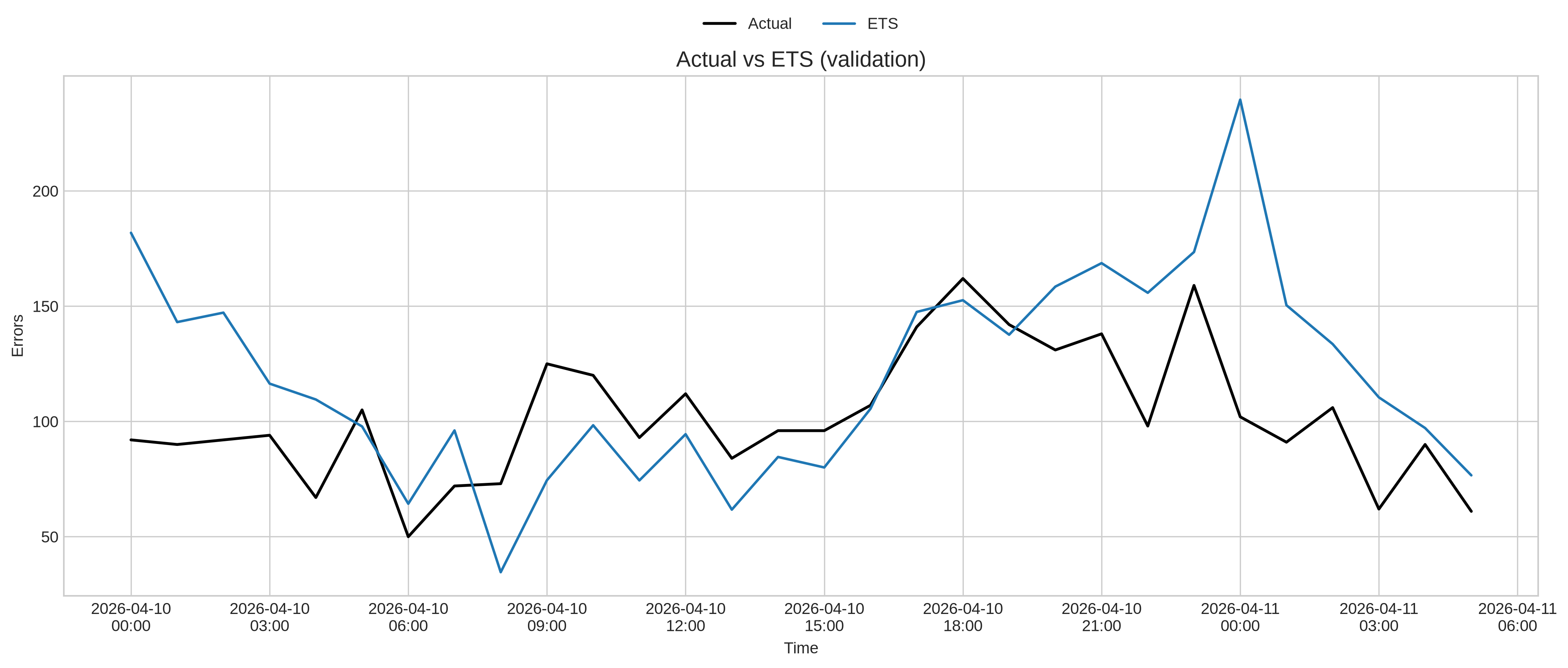
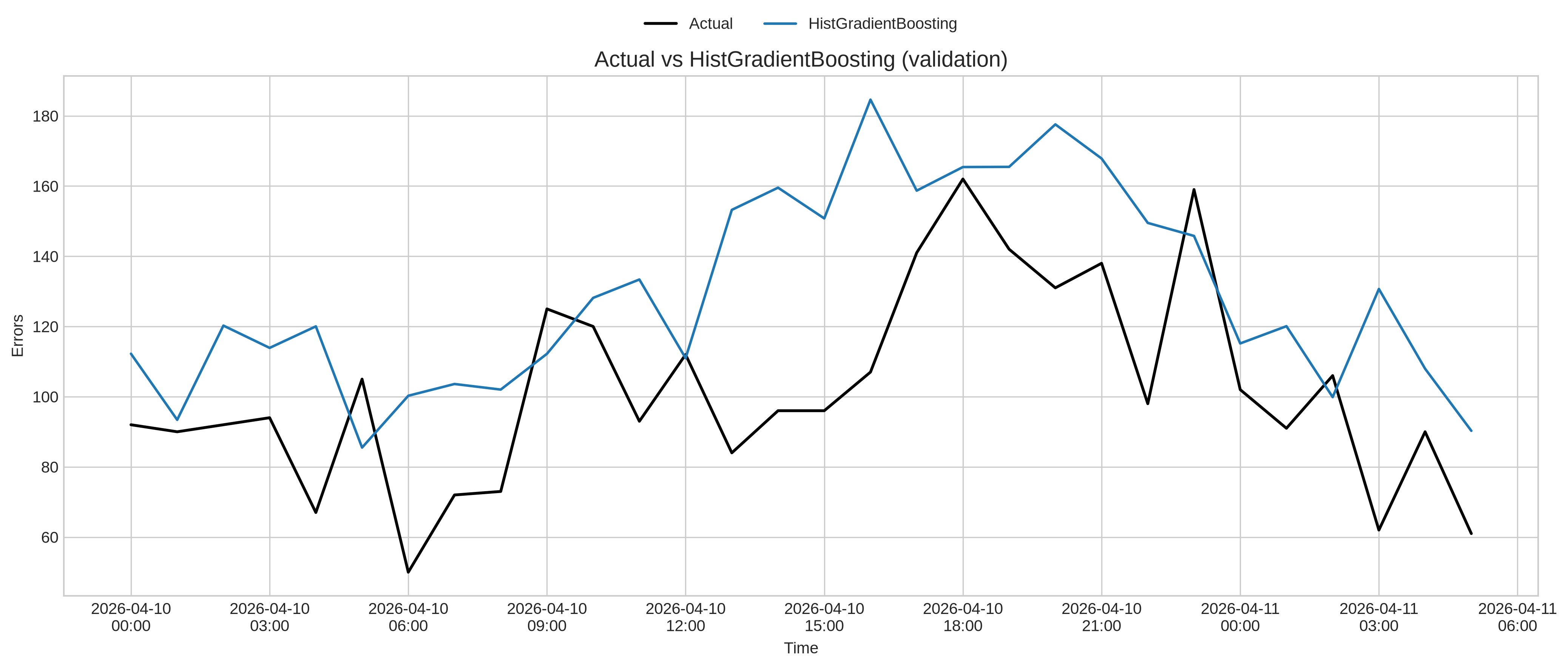
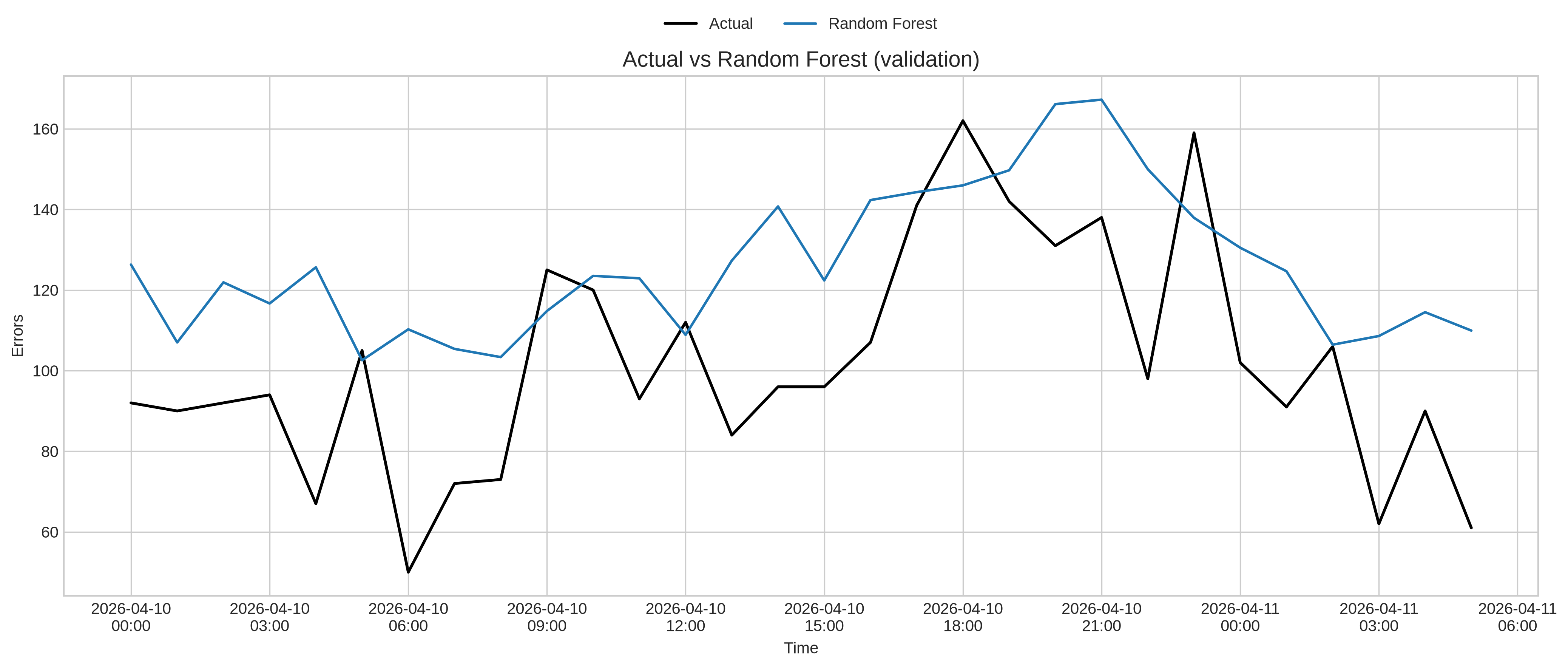
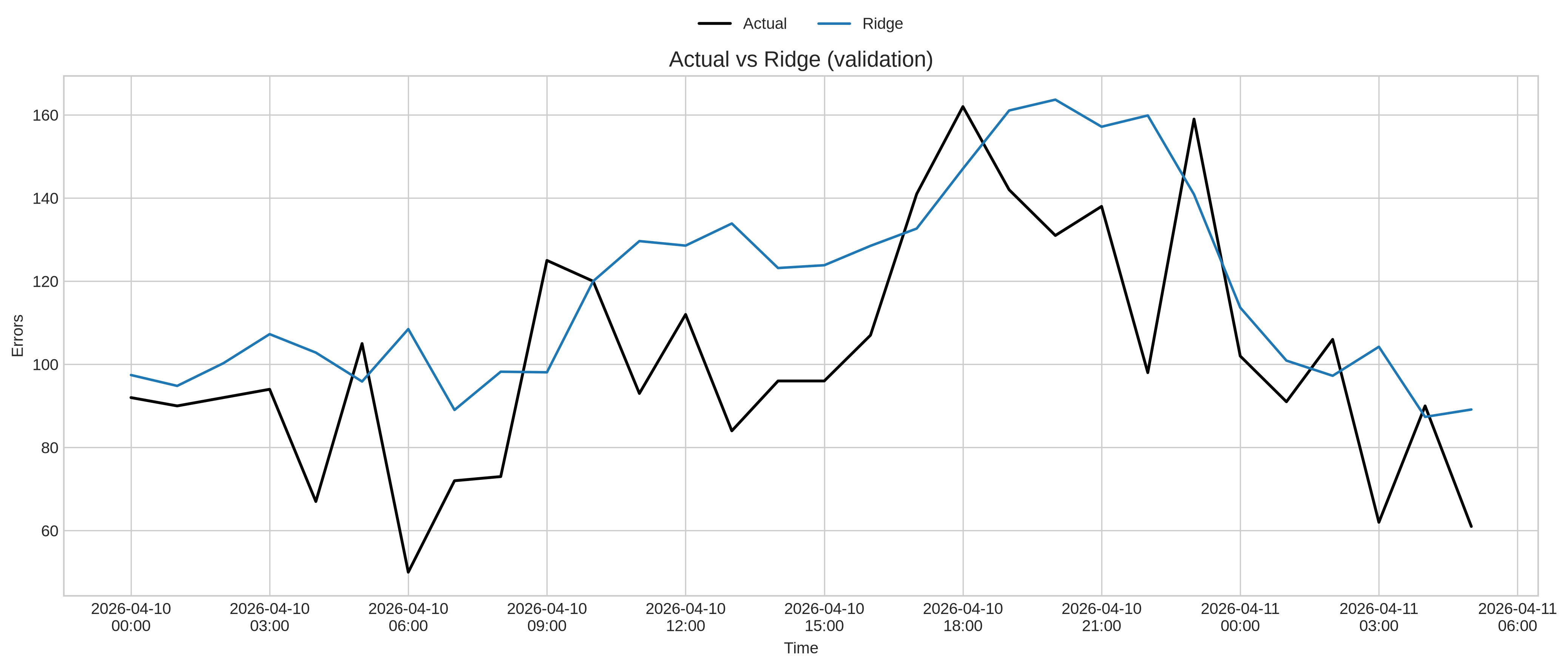
As we can see from our validation visualisations, our models do indeed follow the actual events, but there is a significant amount of variation and a small delay. This is not something that we could have guessed by just looking at the MAE and RMSE results.
This means that even though our ML models may look a lot better in paper, they will not be as good in actual forecasting as our baseline ETS model.
Is There Anything We Can Do?
The answer is yes. We can fine-tune our ML models even further and adjust their features. For example, we can add shorter lags, track rolling means and rolling maxima, and check first differences such as \(y_t - y_{t-1}\) to capture momentum and more, but this is beyond the scope of this article.
Conclusion
In this article, we explored forecasting models that are more flexible and versatile than the simple ETS model we presented in our previous article.
We explained the benefits of these models and the cases in which they are preferable.
We also highlighted that even though ML models offer more flexibility, they are not necessarily the best tool for the job. We need to test, validate, and fine-tune them, and even then pay attention to the details in order to make sure we pick the best forecasting model for our service.