SRE and LLM forecasting
Table of contents
- Introduction
- Forecasting with LLMs
- Setting Up the Experiment
- Preparing the LLM
- Model Results
- Conclusion
Introduction
In this third forecasting article, we will use the concepts introduced in our first and second article about SRE and forecasting, and attempt to expand our toolkit to include large language models in addition to the stochastic and machine learning models presented in the previous articles.
If you have not read those articles yet, I suggest you do so now. This article will reuse and expand on the concepts mentioned in these articles.
Forecasting with LLMs
There are several ways to do forecasting with LLMs, and some are more computationally expensive than others. While researching the topic, I discovered that people at Google have also been thinking along the same lines.
They have released TimesFM (Time Series Foundation Model), a pretrained time-series foundation model developed by Google Research for time-series forecasting. This simplifies our work considerably and makes everything computationally cheaper.
You can find the model repo here. This model is based on a paper presented during ICML 2024 about a decoder-only foundation model for time-series forecasting (arXiv link). This model is based on pretraining a patched-decoder-style attention model on a large time-series corpus and can work well across different forecasting history lengths, prediction lengths, and temporal granularities.
Setting Up the Experiment
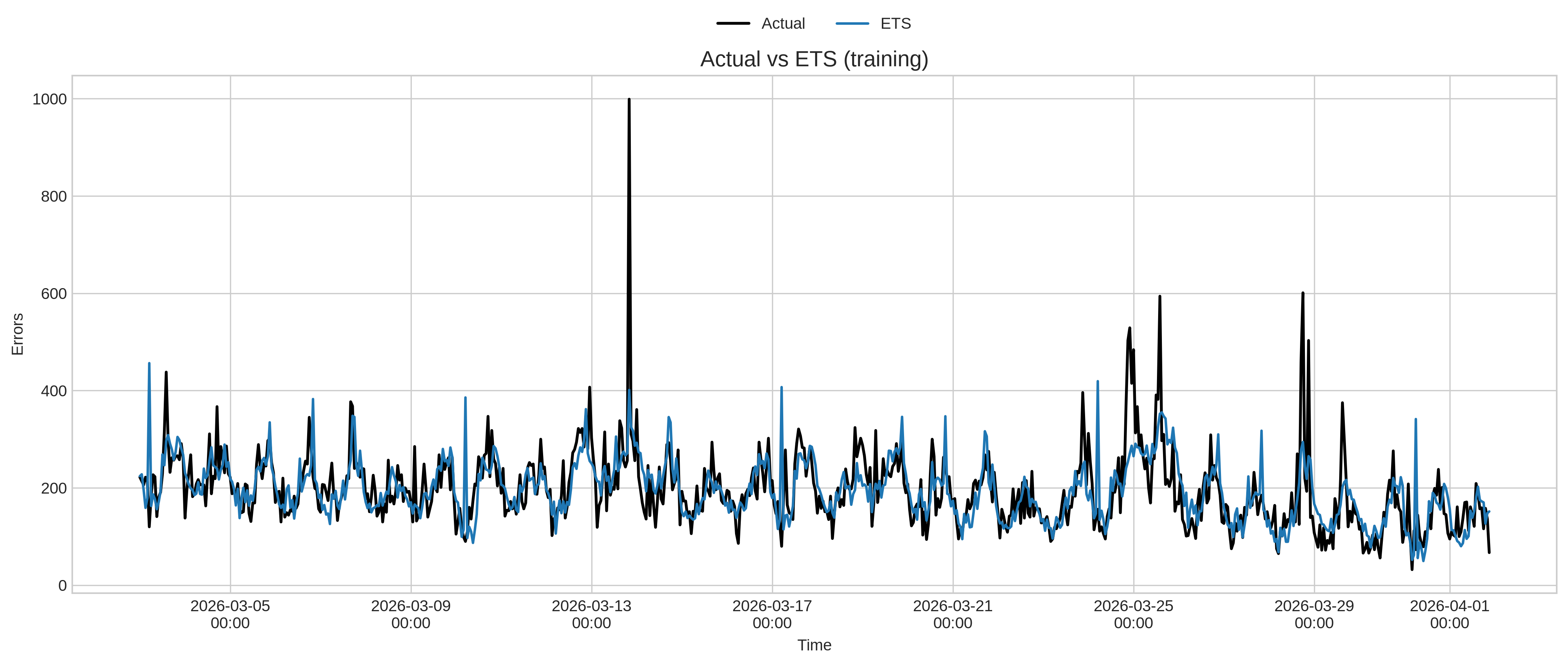
In this article, we will follow the same experimental path as the previous one. In our first article, we identified that our service has a strong seasonality of 168 and established that an ETS stochastic model can capture that quite well.
In the second article, we used this ETS model as our baseline and compared the ML models we evaluated against it. We will do the same in this article, except that instead of ML models, we will use the TimesFM LLM model.
We will use the same dataset included in the previous article and use two methods of evaluation: one using MAE and RMSE and one using visual validation of our results on the validation dataset, which is not part of the model’s training dataset.
As a refresher:
MAE is the average absolute error between the predicted and actual values, expressed in the same units as the data.
RMSE is similar, but it penalizes large errors more heavily, so it is more sensitive to outliers and occasional big misses.
In both cases, lower is better.
ETS Performance
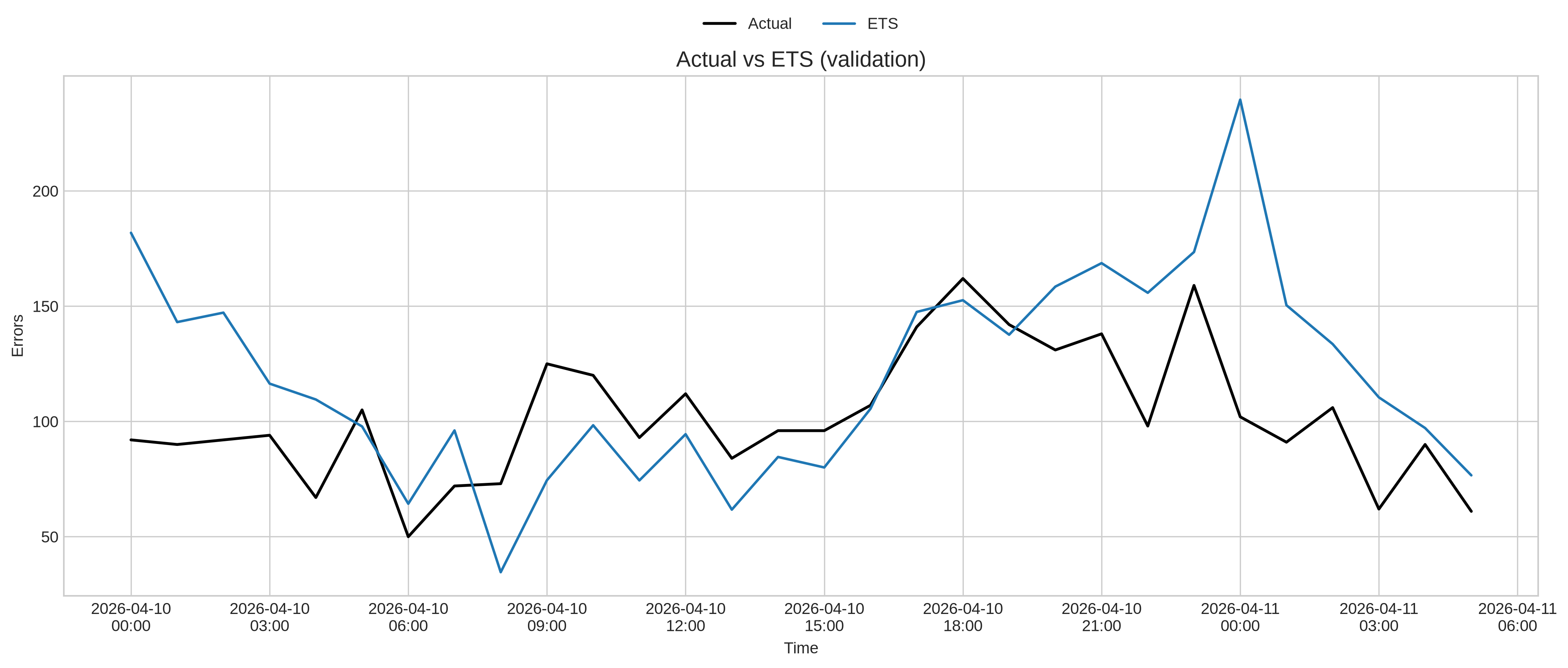
In our previous experiments, we found that ETS produced the following results:
| Split | Model | Rows | MAE | RMSE | Status |
|---|---|---|---|---|---|
| Train | ETS | 717 | 38.98 | 60.52 | Baseline |
| Validation | ETS | 30 | 31.76 | 42.57 | Baseline |
And graphically:
Preparing the LLM
Setting Things Up
In order to use the latest version available to us, we had to clone the Git repository and then execute:
pip install -e ".[torch]"
This installed all the necessary dependencies, as well as the model using the PyTorch backend. This allowed us to work with the 2.5 PyTorch API. To make sure everything was installed properly, we executed:
python - <<'PY'
import timesfm
print(timesfm.__file__)
print([x for x in dir(timesfm) if "Times" in x or "Forecast" in x])
PY
This should output:
['ForecastConfig', 'TimesFM_2p5_200M_torch']
These calls are then used during the model generation phase:
def build_model(context_len: int, max_horizon: int, torch_compile: bool):
    model = timesfm.TimesFM_2p5_200M_torch.from_pretrained(
        "google/timesfm-2.5-200m-pytorch",
        torch_compile=torch_compile,
    )

    model.compile(
        timesfm.ForecastConfig(
            max_context=context_len,
            max_horizon=max_horizon,
            normalize_inputs=True,
            use_continuous_quantile_head=True,
            force_flip_invariance=True,
            infer_is_positive=True,
            fix_quantile_crossing=True,
        )
    )
    return model
This function instantiates the model by downloading the pre-trained model from Hugging Face and caching it locally. The model is quite small compared with other LLMs, and it is roughly 700 MB.
Model Capabilities
At the time of this writing, the latest version of the model is 2.5.
Here is how the model evolved over time:
| Version | Parameters | Max context | Forecast type | Quantile support | Frequency indicator | Horizon notes | Notable changes |
|---|---|---|---|---|---|---|---|
| TimesFM 1.0 | 200M | 512 | Point forecasting | Experimental quantile heads, not calibrated after pretraining | Optional | Any horizon length supported; horizon <= context is recommended but not required | First public checkpoint; univariate forecasting baseline |
| TimesFM 2.0 | 500M | 2,048 | Point forecasting | Experimental 10 quantile heads, not calibrated after pretraining | Optional | Any horizon length supported; horizon <= context is recommended but not required | Larger model, much longer context than 1.0 |
| TimesFM 2.5 | 200M | 16,384 | Point + probabilistic forecasting | Optional 30M continuous quantile head, supports quantile forecasts up to 1,000 horizon | Not required | Public release highlights 1,000-step quantile forecasting and much longer context support | Smaller than 2.0, 8x longer context, improved inference options |
As we can see, version 2.5 is more powerful than the previous versions, and the fact that it supports a 16,384 maximum context makes it ideal for services with larger datasets. In our case, we are using a dataset with 886 hourly buckets, which corresponds to a little less than 37 days. A context window of 16,384 hourly buckets would allow us to load datasets of 682 days, or 22 months.
In addition to this, if we decide to use a period smaller than an hour for our buckets in the case of a very active service, for example if we had a bucket per minute, 16,384 minutes corresponds to 68 days, more than enough for the usual 30-day rolling window commonly used for our default monitoring period.
Furthermore, the latest version is smaller than previous ones and has improved inference options. This has an effect on its performance, as we will see in the next section.
Model Performance
One of the most common issues when it comes to LLM-related work is that it requires a system with a GPU in order to function properly, and some models that support CPUs do not have great performance.
TimesFM is optimised for CPUs as well as GPUs, and during the execution of this experiment, I used an old Toshiba Tecra laptop with the following specs:
Architecture:                            x86_64
CPU op-mode(s):                          32-bit, 64-bit
Address sizes:                           36 bits physical, 48 bits virtual
Byte Order:                              Little Endian
CPU(s):                                  4
On-line CPU(s) list:                     0-3
Vendor ID:                               GenuineIntel
Model name:                              Intel(R) Core(TM) i3 CPU       M 330  @ 2.13GHz
CPU family:                              6
Model:                                   37
Thread(s) per core:                      2
Core(s) per socket:                      2
Socket(s):                               1
Stepping:                                2
CPU(s) scaling MHz:                      96%
CPU max MHz:                             2133,0000
CPU min MHz:                             933,0000
There is no GPU, and:
Mem:           7,5Gi       4,3Gi       435Mi       277Mi       3,4Gi       3,2Gi
Swap:           28Gi       1,6Gi        26Gi
As we can see, the system is an old, low-end business laptop. Nothing performant.
time bash run-model.sh
Validation rows: 30
MAE: 30.4880
RMSE: 34.8226
Wrote output to timesfm_validation_forecast.csv
bash run-model.sh  18,67s user 2,39s system 46% cpu 44,938 total
It executed the forecasting, loading our 886-bucket dataset and forecasting a dataset of 30 buckets in less than 19 seconds. I fully expect that the execution time can be reduced even further if a modern, enterprise-grade system is used.
This is a result that could potentially be used for a variety of services on modest hardware that is readily available. In this case, we did not just forecast one data point, but more than a full day into the future.
Model Results
Numerical Comparison
In our previous execution-time output, we also got the two indicators that we could use to see the actual forecasting performance of our model.
| Split | Model | Rows | MAE | RMSE | Status |
|---|---|---|---|---|---|
| Validation | ETS | 30 | 31.76 | 42.57 | Baseline |
| Validation | TimesFM | 30 | 30.49 | 34.82 | Better (MAE: 4%, RMSE: 18.2%) |
Visual Comparison
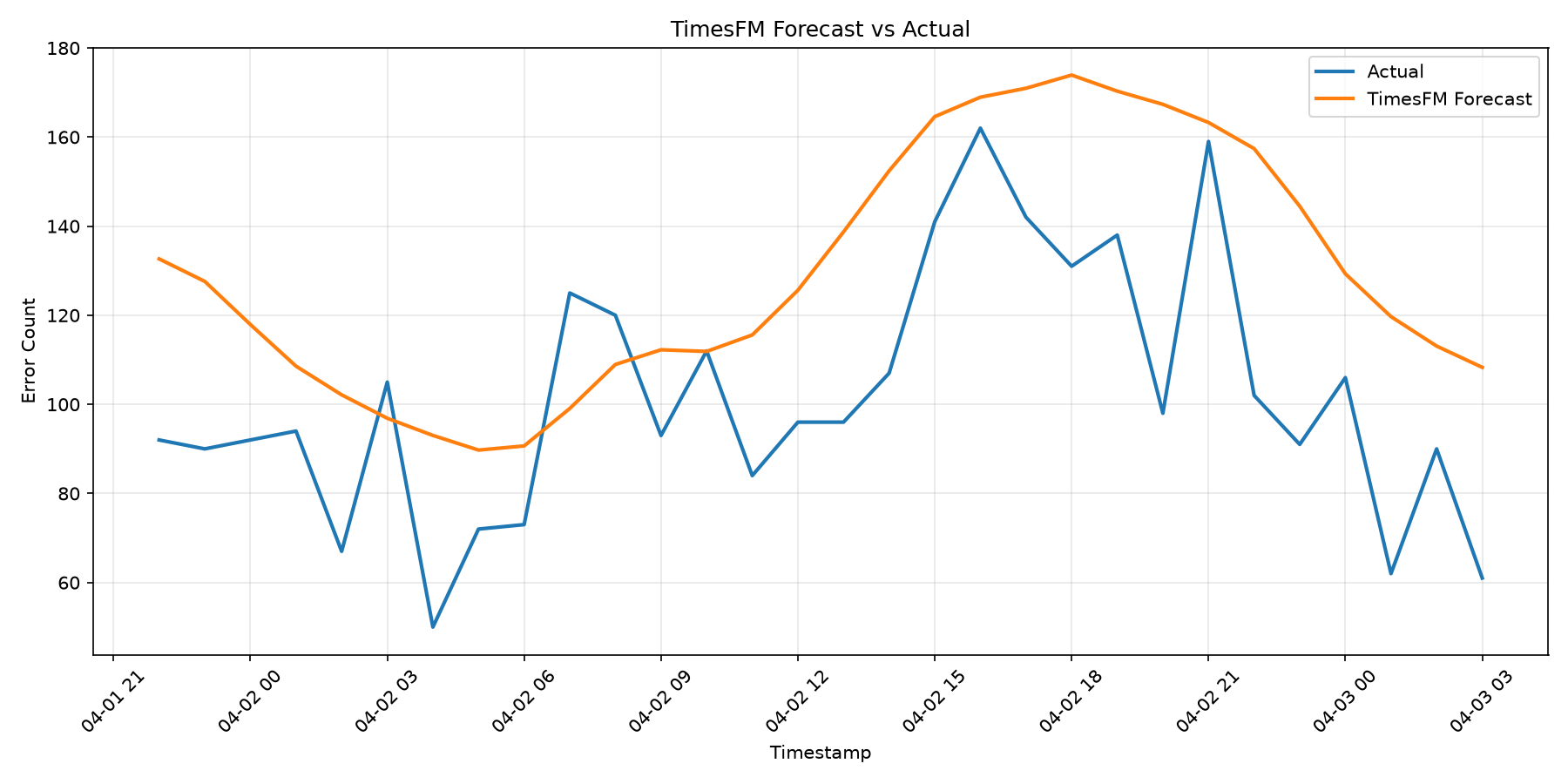
All right, it seems that on paper TimesFM is doing better than ETS, but how does it compare visually?
Let’s see:
Conclusion
In the visual comparison of the two models, we can see that TimesFM forecasting is on par with ETS forecasting. Both models can capture the event trend and can be used to predict the future with a fairly high level of confidence.
So we come now to the question of which model to use. We need to think carefully. ETS will work well for systems that do not change often and show a strong seasonality. ETS will not be able to predict or capture events that happen irregularly and do not follow the seasonal pattern.
On the other hand, the TimesFM LLM will be able to do this. It will be able to capture previous random events and follow their development even if they are irregular and do not follow a seasonal pattern.
We also need to keep in mind that TimesFM supports fine-tuning, which we did not do here. We wanted to capture the performance of the model without any special knowledge of the service and see if it can compete against ETS.
There is room for improvement in these already good results. We also need to keep in mind that even though our services will most likely show some seasonality because they follow human activity, and human activity is tied to the day/night cycle, this is not necessarily always true.
We will have cases where a service does not follow this pattern, and having a flexible solution that can be used to model these services is very important. TimesFM can fill that gap.